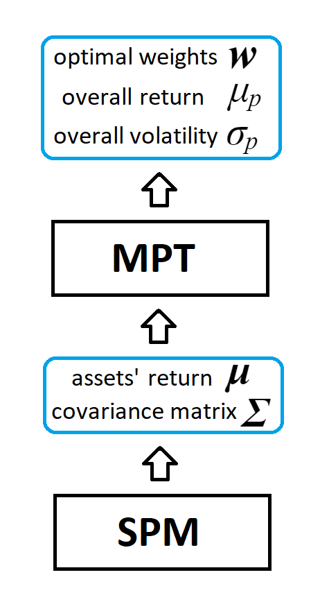
Complementing the Modern Portfolio Theory

The Origin

Given an amount of initial capital, e.g. £1, a bunch of candidate assets (some stocks and optionally a bond), how to distribute your pound upon those assets such that you can take the minimum risk in achieving an expected return at a designated time in future?

This problem led to the proposition of the Modern Portfolio Theory (MPT) in the 1950s. Although over 70 years old, MPT is not a complete theory but rather a framework, and people shall find missing part by themselves.

Key Definitions

Throughout the web-app, the "return" of an asset (e.g. a bond, a stock or a portfolio) is denoted as μ and defined as
μ=V(t) /V(0)
where V(0) is the market value of the asset at time 0 (start time), and V(t) is its market value at time t.
The "risk" of an asset refers to the level of uncertainty of the market value of the asset at a future point of time, which is usually quantified with standard deviation and denoted as σ. Obviously, this uncertainty increases monotonically with the length of time we project in the future.
Meanwhile the "weight" of an asset refers to the asset's market value on the entire portfolio's value at one point of time. We are particularly interested in finding the optimal weights of all candidate assets at time 0, and denote them with a normalised vector w, i.e. ∑wᵢ ≡ wᵀ1 = 1 Thus the entire portfolio's expected return at time t is given by
μₚ = ∑wᵢ μᵢ ≡ wᵀμ with total variance σₚ² derivable from the assets' covariance matrix Σ and weight vectors σₚ² = ∑∑wᵤ σᵤᵥ wᵥ ≡ wᵀΣw
You can also find a list of key definitions associated to a portfolio in the table below.

TERMS	DEFINITION
Expected Return	μₚ ≔wᵀμ
Standard Deviation	σₚ ≔ √(wᵀΣw)
Sharpe Ratio	Sₚ ≔ ( μₚ - 1 ) / σₚ if no bond, or Sₚ ≔ ( μₚ - μ₀ ) / σₚ if a bond is included
Lever	ℰₚ ≔ ∑|wᵢ|, i ≥ 0, a.k.a. risk exposure
Tangency Portfolio	If ∃(Cᵗᶢ > 0) and C ← Cᵗᶢ then w₀ = 0, i.e. zero bond position
Non-shortselling Solutions	Exist iff ∃C ∀i wᵢ ≥ 0

Two Technical Pillars

There are two steps in deriving minimum-risk solutions, including a model-fitting step and an extrema-finding step. Correspondingly, there are two technical pillars underpinning - stochastic process modelling (SPM) and MPT itself.
H. Markowitz (1927 - 2023) , the founding contributor of the MPT, showed that given a number of risky assets with (or without) a risk-free bond, if we know each risky asset's expected return, volatility and covariance between each two of them, we may exploit this and set up a combination that minimises the total risk given a fixed expected total return. In other words, an optimal combination of the candidate assets may effectively cancel some volatilities between each other and reduce the overall uncertainty to a minimum.
However, MPT doesn't tell people how to estimate risky assets' expected returns and associated covariance matrices. As these quantities have always been evolving in time, we may resort to the second technical pillar- SPM, and predict them at a level of confidence. e-Gauss currently employs two SP models in fitting - DBM (drifted Brownian motion for asset log-returns) and DOU (dynamically over/under-valued). DBM is popular in the investment banking industry for financial asset pricing, e.g. in the Black-Scholes model. DOU is my home-made and favorite, which works similar to DBM and takes market efficiency as a new parameter into account.
Lastly, why is this app named e-Gauss? Because both DBM and DOU are Gaussian process.

Algorithm of finding the extrema

The solution is to find the weight vector w that minimises the corresponding Lagrangian multiplier ℒ, i.e.

argmin_wℒ(w)
where if bond is excluded
ℒ(w) ≔wᵀΣw·C/2 - wᵀμ + λ (wᵀ1 - 1)
≡ σₚ²·C/2 - μₚ + λ (wᵀ1 - 1) else if a bond is included ℒ(w) ≔ wᵀΣw·C/2 - wᵀμ - w₀μ₀ + λ(w₀+wᵀ1 - 1)

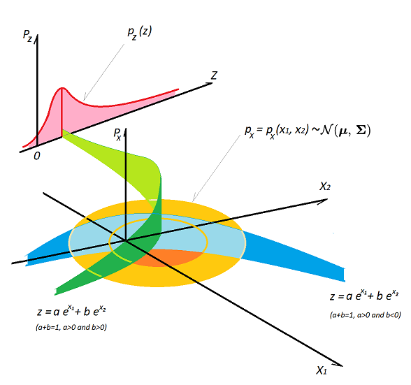
Return Distribution on Maturity

Though we cannot predict the exact market value of any risky asset at a future time, it is possible to figure out the distribution.

The figure below provides an example - a graphical interpretation on calculating the density function of the value of a portfolio, p(z). The portfolio consists of only 2 stocks with initial capital weight a and b respectively, while the two stocks' log-return on maturity are denoted as X₁ and X₂, supposedly being two correlated Gaussians.



Back